
RESEPT: a deep-learning framework for characterizing and visualizing tissue architecture from spatially resolved transcriptomics
Published:
Motivation
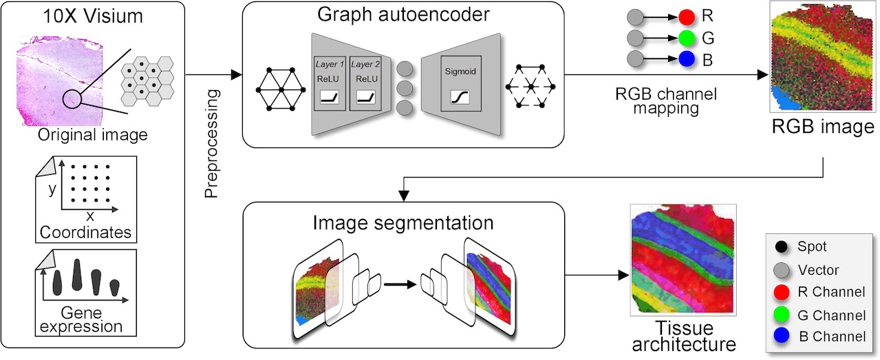
patially resolved transcriptomics provides a new way to define spatial contexts and understand the pathogenesis of complex human diseases. Although some computational frameworks can characterize spatial context via various clustering methods, the detailed spatial architectures and functional zonation often cannot be revealed and localized due to the limited capacities of associating spatial information. We present RESEPT, a deep-learning framework for characterizing and visualizing tissue architecture from spatially resolved transcriptomics. Given inputs such as gene expression or RNA velocity, RESEPT learns a three-dimensional embedding with a spatial retained graph neural network from spatial transcriptomics. The embedding is then visualized by mapping into color channels in an RGB image and segmented with a supervised convolutional neural network model.
The RESEPT framework
(a) A spatial retained spot graph is established by spatial distances of spots and their expression or velocity matrix. The graph autoencoder takes the adjacent distance matrix of the spot graph as the input. Its encoder learns a 3-dimensional embedding of a spatial cell graph. The decoder reconstructs the adjacent correlations among all cells by dot products of the 3-dimensional embeddings followed by a sigmoid activation function. The graph autoencoder is trained by minimizing the cross-entropy loss between the input spatial and the reconstructed graphs. The learned 3-dimensional embeddings are mapped to a full-color spectrum to generate an RGB image revealing the spatial architecture. (b) The segmentation model takes the RGB image as the input, which may be processed with an imputation operation if missing spots exist. Its backbone network ResNet101 consists of one convolutional layer and a series of residual blocks, in which one type of residual block named convolutional block stacks three convolutional layers with a convolutional skip connection from the input signals to the output feature maps. The other type of residual block identity block stacks three convolutional layers with a direct skip connection from the input signals to the output feature maps. This extra deep network firstly extracts rich visual features of the input image. The encoder module further extracts multi-scale semantic features by applying four atrous convolutional with different rates and sizes of filters and one global pooling layer to the basic visual feature maps. And the decoder module up-samples the multi-scale features to the same size with basic visual feature maps and then concatenates them together. After a softmax activation function, the decoder module outputs a segmentation map classifying each spot into a specific spatial architecture. 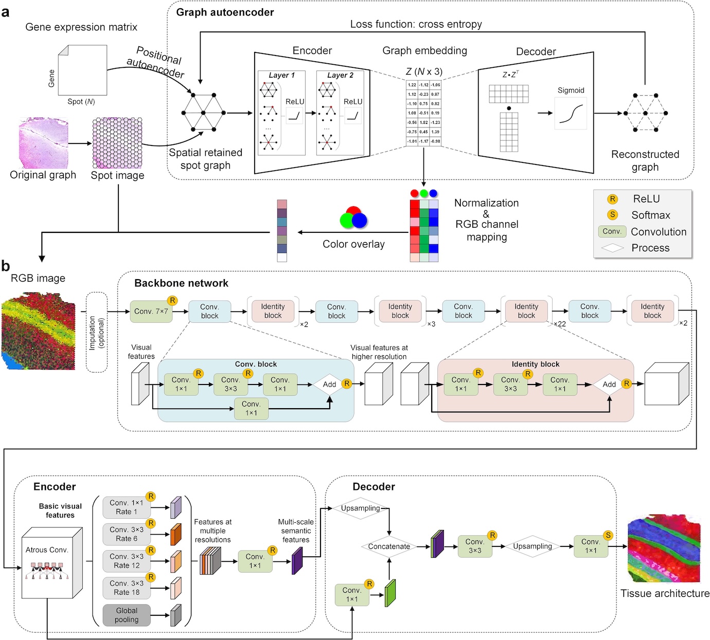
The RESEPT workflow and performance.
(a) Mean and standard deviation of sequencing reads of 17 human brain datasets on 10x Visium platform. CT1 to 151,508 have manual annotations as the benchmark, CT2 & 151,674 for simulation for high mean and low standard deviations of read depth, G1, AD1, and AD2 for the case studies (more details in Supplementary Tables 1–2). (b) Performance of tissue architecture (with 7 clusters pre-defined) identification by seven existing tools and RESEPT on criteria ARI. (c) Stability of tissue architecture identification across sequencing depths on samples CT2 using different tools. The Y-axis shows ARI performance, and the X-axis represents the sequencing depth with subsampling. The lines are smoothed by the B-Spline smooth method. (d) Normalized performance vs sequencing depth on sample CT2. Performance of full sequencing depth is set as 1.0. RESEPT_E1 using the scGNN embedding, RESEPT_E2 using the spaGCN embedding. (e) and (f) The stability of ARI and normalized performance against the grid sequencing depth for samples CT2 and 151674. CT2 and AD2 results of HMRF were excluded due to failure to produce outcomes. (g) Ground truth of AD2. (h) Spatial domains on AD2 detected by RESEPT. (i) – (n) Tissue architecture results based on BayesSpace, Seurat, Giotto, stLearn, and SpaGCN, respectively. 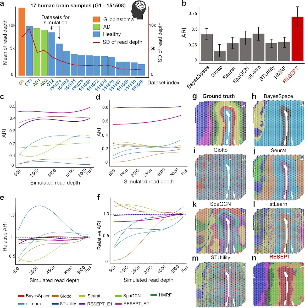
Model interpretation and generalizability for RESEPT
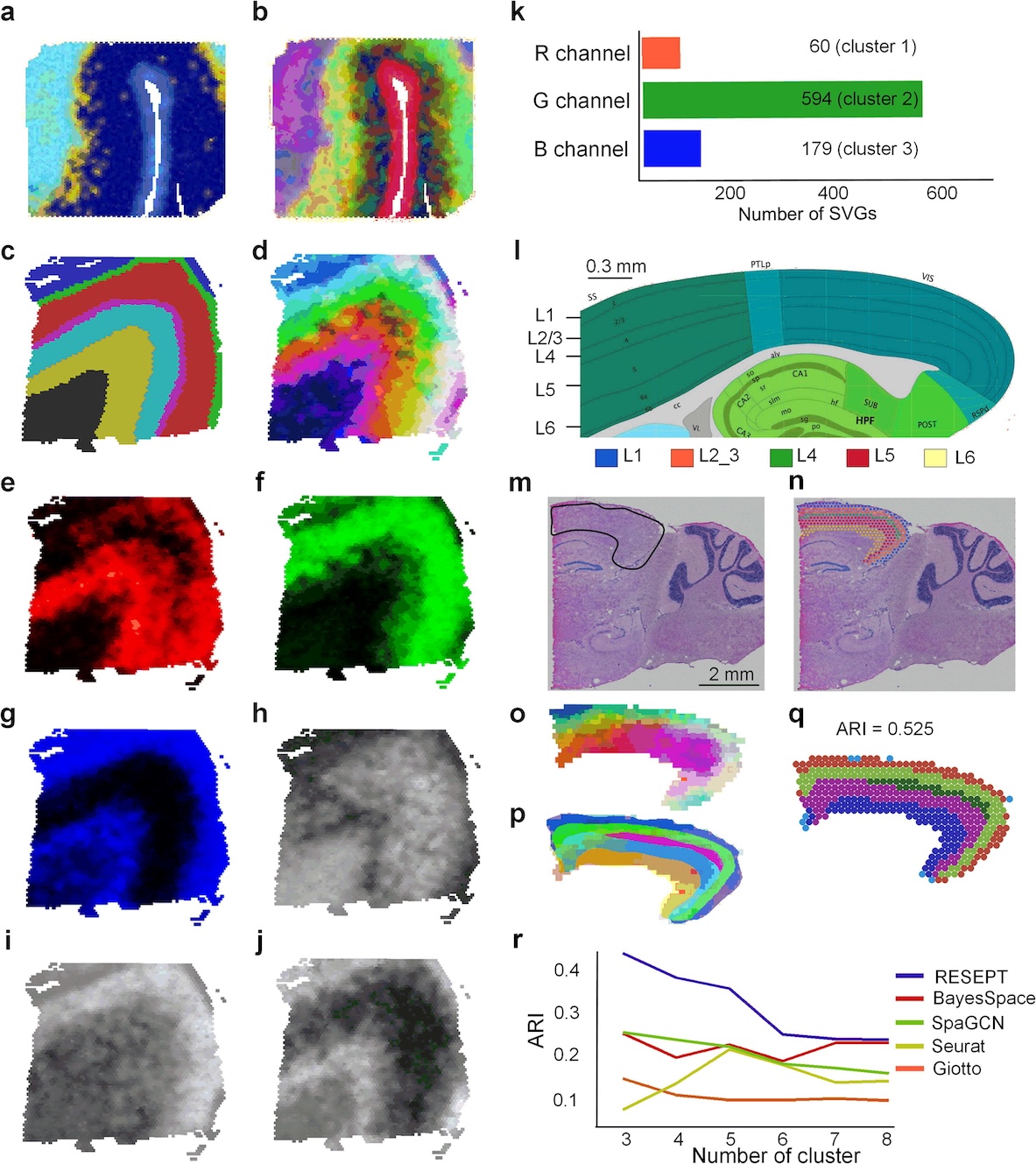
(a) RGB image generated from expression value (Moran’s I = 0.787). (b) RGB image generated from RNA velocity (Moran’s I = 0.920). (c) The figure Shows the ground truth of the 151,673 sample. (d) The RGB image was reconstructed from whole transcriptomics. (e) Visualization of Red channel from sample 151673′s reconstructed RGB image. (f) Visualization of Green channel from sample 151673′s reconstructed RGB image. (g) Visualization of Blue channel from sample 151673′s reconstructed RGB image. (h-j) Grayscale images reconstructed from genes in clusters 1–3 by k-means clustering, respectively. (k) Number of SVGs mapped on RGB channels, where the Red channel corresponds to 60 genes from cluster 3, the Green channel corresponds to 594 genes from cluster 1, and the Blue channel corresponds to 179 genes from cluster 2. (l) Mouse brain sagittal section from the Allen Brain Atlas [57]. (m) The mouse brain cortex region was cropped from the mouse brain sagittal posterior at the 10x official website (the region in black line). (n) The cropped mouse cortex was labeled based on annotation from the Allen Brain Atlas in figure panel l, where Blue represents layer 1, orange represents layers 2 and 3, Green represents layers 4 and 5, and Red represents layer 6 [14]. (o) The RGB image was reconstructed based on the mouse cortex transcriptome. (p) RESEPT’s results as a segmented image from the mouse brain cortex (ARI 0.336). (q) The figure shows ARI and spot-level RESEPT segmentation results. (r) The figure shows the impact of cluster numbers in human breast cancer (1160920F) results, where the x-axis is the number of predicted clusters and the y-axis indicates the ARI score. HMRF, stLearn, and STutility were excluded because of failing to find 3 to 8 clusters.
RESEPT identifies spatial cellular patterns in the human postmortem middle temporal gyrus (MTG)
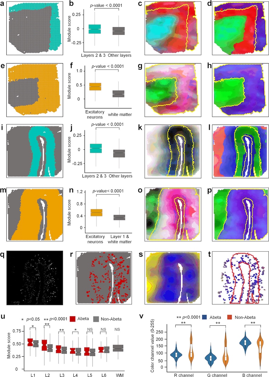
(a) Layers 2 and 3 (cyan) of sample AD1. (b) The module score of the cortical layers 2 and 3 and other layers from sample AD1, where the x-axis shows layer categories and the y-axis represents scores. (c) RGB images where the yellow line points out the ground truth of layers 2 and 3 for samples AD1. (d) The segmented images were reconstructed by setting the number of segments as three for AD1. (e) Layers 2 to 6 architecture (yellow) of AD1, where excitatory neuron cells are distributed. (f) The module score of the cortical layers 2 to 6 and white matter for sample AD1, where the x-axis shows layer categories and the y-axis represents scores. (g) RGB images of AD1 were reconstructed from excitatory neuron cell markers. (h) The segmentation images via selecting the number of segments as two for samples AD1. (i)-(p) Similar analyses for AD2. (q) Aβ plaques are located by immunofluorescence assay. (r) The spots with the accumulation of Aβ plaques in red color. (s) Reconstructed RGB image from 20 genes relevant to the Aβ region. (t) Reconstructed RGB image cropped according to the Aβ region and marked by layers 2&3 (encircled by the red line). (u) The module score regarding the Aβ region and non-Aβ region for each layer, where red color represents the Aβ region, and gray color represents the non-Aβ region. (v) RGB channels show the color value dispersion, where the violin in the blue color represents RGB values in the Aβ region, and the violin in the orange color represents RGB values in the non-Aβ region.
RESEPT identifies tumor regions in glioblastoma samples
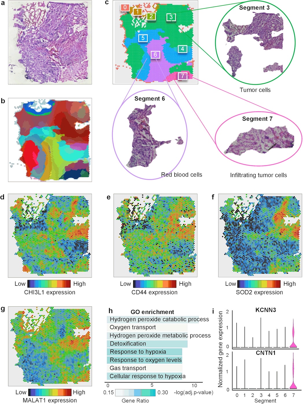
(a) Original H&E staining image from the 10x Genomics. (b) Tissue architecture was identified via the RESEPT pipeline. (c) Labeled segmentation by RESEPT and Segments 3, 6, and 7 are cropped according to the segmentation result. Based on morphological features, our physiologist found Segment 3 contains large tumors from morphological features; Segment 6 contains a large number of blood cells; Segment 7 contains infiltrating tumor cells. (d), (e), (f), and (g) show the expression of Glioblastoma markers CHI3L1, CD44, SOD2, and MALAT1 in all spots based on the logCPM normalization value. (h) The bar plot shows the results of GO enrichment analysis, indicating Segment 6 has a large proportion of blood cells with blood signature genes for gas transport. (i) Infiltrating glioblastoma signature marker genes KCNN3 and CNTN1 are highly expressed in Segment 7 based on the logCPM normalization.
GitHub link
https://github.com/OSU-BMBL/RESEPT
Related Publications
$Chang, Yuzhou, Fei He, Juexin Wang, Shuo Chen, Jingyi Li, Jixin Liu, Yang Yu et al. “Define and visualize pathological architectures of human tissues from spatially resolved transcriptomics using deep learning.” Computational and structural biotechnology journal 20 (2022): 4600-4617.
$Yuzhou Chang, Fei He and Juexin Wang contributed equally to the paper as the first authors.